5.7 KiB
| title | date | description | hero | author | menu | tags | categories | |||||||||||||
|---|---|---|---|---|---|---|---|---|---|---|---|---|---|---|---|---|---|---|---|---|
| Mobile Manipulation | 2024-12-30T09:00:00+00:00 | Introduction to Sample Post | images/kavar_background.jpg |
|
|
|
|
This project incorporates several robotics concepts to perform a pick and place task in simulation using a mecanum-wheeled mobile robot with a 5 degree-of-freedom robot arm.
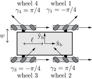
Omnidirectional Mobile Base Kinematics (Mecanum Wheels)
This robot uses mecanum wheels, which are omnidirectional wheels with 45-degree rollers that allow the robot to move in any direction without changing its orientation. When controlling the robot, we command the wheel velocities, which can be described by the following equation:
u_i=\frac{1}{r_i}\overbrace{\begin{bmatrix}1 & \tan\gamma_i\end{bmatrix}}^{\text{driving direction}}\underbrace{\begin{bmatrix}\cos\beta_i & \sin\beta_i \\ -\sin\beta_i & \cos\beta_i\end{bmatrix}}_{\text{linear velocity in wheel frame}}
\overbrace{\begin{bmatrix}-y_i & 1 & 0 \\ x_i & 0 & 1\end{bmatrix}}^{\text{linear velocity in body frame}} V_b
where:
- \(u_i\) is the wheel velocity
- \(r_i\) is the wheel radius
- \(\gamma_i\) is the angle of the roller relative to the wheel's driving direction
- \(\beta_i\) is the angle of the wheel relative to the robot's x-axis
- \(x_i\) and \(y_i\) are the x and y coordinates of the wheel relative to the robot's center
- \(V_b\) is the robot's 3D body twist, composed of the linear and angular velocity: \([v_x, v_y, \omega]\)
Odometry
Odometry is the process of estimating the mobile robot's pose by integrating the wheel velocities. The robot's pose is represented by the chassis configuration \([\phi, x, y]\), where \(\phi\) is the orientation and \(x, y\) are the position in the world frame.
The odometry function computes the new chassis configuration based on the difference between the current and previous wheel configurations assuming a constant velocity between the two wheel configurations.
def odometry(chassis_config: np.array, delta_wheel_config: np.array) -> np.array:
    """
    Using Odometry, a new chassis configuration is computed based on the
    difference between the current and the previous wheel configuration.

    Args:
        chassis_config (np.array): The current chassis configuration [phi, x, y]
        delta_wheel_config (np.array): The difference in wheel configuration

    Returns:
        np.array: The new chassis configuration [phi, x, y]
    """
    phi, x, y = chassis_config
    # delta_theta is the difference in wheel angles
    # Since we are assuming constant wheel speeds, dt = 1
    dt = 1  # Use actual timestep between wheel displacements for non-constant speeds
    theta_dot = delta_wheel_config / dt
    # Calculate the Body twist using the pinv(H0) and theta_dot
    V_b = RC.F @ theta_dot
    # Integrate to get the displacement: T_bk = exp([V_b6])
    V_b6 = np.array([0, 0, *V_b, 0])
    T_bk = mr.MatrixExp6(mr.VecTose3(V_b6))
    T_sk = RC.T_sb(phi, x, y) @ T_bk
    new_phi = np.arctan2(T_sk[1, 0], T_sk[0, 0])
    new_chassis_config = np.array([
        new_phi,
        T_sk[0, 3],
        T_sk[1, 3]
    ])
    return new_chassis_config
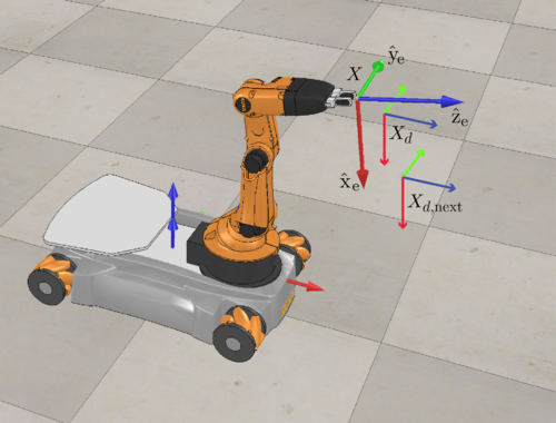
Task-Space Feedforward & Feedback Control
To perform the pick and place task, we need to implement a control law that can track a desired end-effector trajectory. The control law is given by:
V_e(t) = \overbrace{[Ad_{X^{-1}X_d}]V_d(t)}^{\text{Feedforward}} + K_pX_{err}(t) + K_i \int X_{err}(t)
where:
- \(V_e(t)\) is the error twist required to track the desired trajectory
- \(X\) is the current end-effector configuration
- \(X_d\) is the desired end-effector configuration
- \(V_d(t)\) is the desired end-effector twist
- \(K_p\) is the proportional gain matrix
- \(K_i\) is the integral gain matrix
- \(X_{err}(t)\) is the error between the current and desired end-effector configurations
def feedback_control(X, Xd, Xd_next, Kp, Ki, control_type: str = 'FF+PI', dt: float = 0.01) -> tuple:
    """
    Calculate the kinematic task-space feedforward plus feedback control law.
    V(t) = [Adjoint(inv(X)*Xd)]V_d(t) + Kp*X_err(t) + Ki*integral(X_err(t))
    Args:
        X (np.array): The current actual end-effector configuration (T_se)
        Xd (np.array): The current end-effector reference configuration (T_se,d)
        Xd_next (np.array): The end-effector reference configuration at the next timestep in the reference trajectory
        Kp (np.array): The Proportional gain matrix
        Ki (np.array): The Integral gain matrix
        control_type (str, optional): The type of simulation. Defaults to 'FF+PI'. ['FF+PI', 'P', 'PI']
        dt (float, optional): The timestep between reference trajectory configs. Defaults to 0.01.
    Returns:
        tuple: A tuple containing the twist V and the error X_err
    """
    X_err = mr.se3ToVec(mr.MatrixLog6(mr.TransInv(X) @ Xd))
    # print(f'X_err:\n{np.round(X_err, 3)}')
    Vd = mr.se3ToVec((1/dt) * mr.MatrixLog6(mr.TransInv(Xd) @ Xd_next))
    # print(f'Vd:\n{np.round(Vd, 3)}')
    if control_type == 'FF+PI':
        V = mr.Adjoint(mr.TransInv(X) @ Xd) @ Vd + \
            (Kp @ X_err) + (Ki @ (X_err * dt))
    elif control_type == 'P':
        V = (Kp @ X_err)
    elif control_type == 'PI':
        V = (Kp @ X_err) + (Ki @ (X_err * dt))
    else:
        print(f'Invalid sim_type: {control_type}, using FF+PI')
        V = mr.Adjoint(mr.TransInv(X) @ Xd) @ Vd + \
            (Kp @ X_err) + (Ki @ (X_err * dt))
    # print(f'V:\n{np.round(V, 3)}')
    return V, X_err